Apache Iggy - Kafka Muadili Ancak Protokol Uyumlu Değil

Giriş

Rust ile geliştirilmiş. Aynı Kafka gibi şu kavramlara sahip

• Streams
• Topics
• Partitions
• Producers
• Consumers

Apache Pinot vs ClickHouse vs Snowflake

Giriş

Açıklaması şöyle

Apache Pinot vs ClickHouse vs Snowflake

On the surface, Apache Pinot, ClickHouse, and Snowflake all look like fast SQL engines. But in reality, they were built for three completely different execution models. Understanding this is the difference between building a system that works and one that collapses under load.

Snowflake: The Analytical Brain

Snowflake is designed for: • Large joins • Complex SQL • Batch loaded data • A small number of heavy users

It is optimized for throughput, not concurrency. Snowflake expects: • A few analysts • Running long queries • Scanning lots of data

Thus, it makes Snowflake perfect for reporting, finance, and BI. It is terrible for powering APIs or live product features. When 1,000 users refresh a dashboard, Snowflake spins up 1,000 warehouses. This is expensive and slow. Snowflake answers: "What happened?"

ClickHouse: The Fast Scanner

ClickHouse is a blazing-fast OLAP engine. It is built for: • Huge event tables • Fast scans • Aggregations • Ad hoc exploration

ClickHouse is amazing when you want to: • Explore data • Run heavy group by queries • Scan billions of rows

But ClickHouse still assumes dozens of users and queries that tolerate seconds. It does not handle: • Extreme concurrency • Streaming freshness • Hybrid real-time plus batch queries

ClickHouse answers: "What is happening?"

Apache Pinot: The Decision Engine

Pinot is built for something else entirely. It is designed for: • Thousands of concurrent queries • Millisecond response times • Streaming ingestion • Product and API workloads

Pinot assumes: • Every click triggers a query • Every price change is computed live • Every ML system needs fresh features

Pinot does not scan tables, but it navigates segments, indexes, and StarTrees to avoid touching most data. Pinot answers: "What should the product do next?"

Apache Pinot - Bir OLAP veri tabanı - What is Happening

Giriş

Açıklaması şöyle. Yani LinkedIn şirketinde yaratılmış. LinkedIn şirketinde ilk olarak User-facing analytics özelliklerinden olan ‘Who Viewed My Profile?’ ve ‘Talent Search’ gibi işler için kullanılmış

Apache Pinot was created, as was Kafka, at LinkedIn to power analytics for business metrics and user facing dashboards. Since then, it has evolved into the most performant and scalable analytics platform for high-throughput event-driven data.

Uber

Apache Pinot'un petabyte büyüklüğünde veriyi rahatlıkla işleyebileceği duyulunca, ilk önce  “Restaurant Manager" paneli için kullanılmış. Şu anda fiyatlandırma için kullanılıyor. Açıklaması şöyle

Uber does not run analytics for reporting. It runs analytics to decide how much a ride costs, how quickly a driver gets matched, how incentives shift, and how supply and demand are balanced while the customer is still on the screen.

This is the reason Uber runs around 600 million Apache Pinot queries every day, which works out to roughly 7,000 queries per second on more than 20 petabytes of data. These are not batch jobs or delayed dashboards. These are live, operational queries sitting directly in the critical path of the product.

Apache Pinot Nedir ?

Açıklaması şöyle. Bir OLAP veri tabanı ancak bir sürü kaynaktan veri çekebiliyor. Yani hem tarihsel hem de gerçek zamanlı kaynaklardan veri çekebiliyor ve bunları SQL ile sorgulayabilmemizi sağlıyor

Apache Pinot is a distributed OLAP store that can data from various sources such as Kafka, HDFS, S3, GCS, and so on and make it available for querying in real-time. It also features a variety of intelligent indexing techniques and pre-aggregation techniques for low latency.

Cevaplar hızlı ve güncel. Açıklaması şöyle

Answers contain fresh data — As soon as the data is ingested, Pinot makes them available for querying, typically within seconds. So, you won’t get any stale data in the answers.

Answers will be quick — Pinot makes sure that you will always get an answer within milliseconds of latency, even though it is super busy or having to scan billions of records to find the answer.

Can answer multiple questions concurrently — You may not be the only one querying Pinot. It could be hundreds or even millions of users querying Pinot concurrently. But Pinot makes sure that it scales and be available to accommodate all that questions.

Açıklaması şöyle

Pinot is the wrong tool when you need :

i. Large multi-table joins Pinot is optimized for fast scans and aggregations on single denormalized tables. It is not a relational engine.

ii. Exploratory data science Ad hoc queries that scan large parts of the dataset, join many tables, and change constantly belong in a warehouse or notebook environment.

iii. Analyst-driven BI workflows If your workload is dominated by a few people running complex SQL with unpredictable shapes, Pinot is not what you want.

iv. Complex SQL pipelines CTEs, window functions, and deep transformations are not what Pinot is built to do.

Lambda Architecture

Açıklaması şöyle

Pinot follows the lambda architecture. It supports near-real-time data ingestion by consuming online data directly from Kafka and offline data from the Hadoop system. Offline data will serve as a global view, while online data will provide a more real-time view.

Açıklaması şöyle

In most data stacks, data flows like this:

Events → Kafka → Data lake → Warehouse → BI → Decisions

By the time anyone looks at the data, the moment is already gone. Pinot flips that model. With Pinot, data flows like this:

Events → Kafka → Pinot → APIs → Product, pricing, alerts, ML systems

Pinot Hangi Problemleri Çözer?

1. User-facing analytics

Dashboards ve Personalization için kullanılır

Açıklaması şöyle

Dashboards — Pinot has been purpose-built to power user-facing applications and dashboards that are supposed to be accessed by millions of users concurrently. While doing so, Pinot maintains stringent SLAs, which are typically in milliseconds range to ensure a pleasant user experience.

Personalization — Apart from that, Pinot is good at performing real-time content recommendations. For example, Pinot powers the news feed of a LinkedIn user, which is based on the impression discounting technique. You can feed clickstream, view stream, and user activity data to Pinot to generate content recommendations on the fly.

2. Ad-hoc querying and exploratory data analysis

Data analysts ve Data scientists tarafından kullanılır

3. Operational intelligence and time-series data processing

Time-series database (TSDB) olarak kullanılır

Storage Nasıldır?

Açıklaması şöyle. Columnar storage kullanıyor

Under the covers, it features columnar storage with intelligent indexing techniques and pre-aggregation techniques. Thus, making Pinot an ideal choice for real-time, low-latency OLAP workloads. For example, BI dashboards, fraud detection, and ad-hoc data analysis are few use cases where Pinot excels.

Açıklaması şöyle

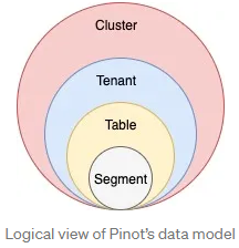
Segments — Raw data ingested by Pinot is broken into small data shards, and each shard is converted into a unit known as a segment. A segment is the centerpiece in Pinot’s architecture which controls data storage, replication, and scaling.

Tables and schemas — One or more segments form a table, which is the logical container for querying Pinot using SQL/PQL. A table has rows, columns, and a schema that defines the columns and their data types.

Tenants — A table is associated with a tenant. All tables belonging to a particular logical namespace are grouped under a single tenant name and isolated from other tenants.

If you are familiar with log-structured storage like Kafka, a segment resembles a physical partition while a table represents a topic. Both topics and tables expect to grow infinitely over time. Therefore, they are partitioned into smaller units so that they can be distributed across multiple nodes.

Şeklen şöyle

Mimarisel Bileşenleri Nelerdir?

Şeklen şöyle

Bileşenler

Açıklaması şöyle. Yukarıdaki şekilde Broker, Server ve Controller görülebilir.

A typical Pinot cluster has multiple distributed system components: Controller, Broker, Server, and Minion. In production, they are deployed independently for scalability. 

1. Pinot Broker

Açıklaması şöyle. Sorguları işleyen bileşen

Brokers are the components that handle Pinot queries. They accept queries from clients and forward them to the right servers. They collect results from the servers and consolidate them into a single response to send it back to the client.

Broker sorgunun  scatter-gather şeklinde çalışmasını sağlar. Açıklaması şöyle.

Pinot executes queries in a scatter-gather manner instead of the databases that leverage the materialized views where query result has been precomputed.

Scatter-gather execution model Nedir?

Açıklaması şöyle.

Queries are received by brokers — which checks the request against the segment-to-server routing table — scattering the request between real-time and offline servers.

The two servers then process the request by filtering and aggregating the queried data, then returned to the broker. Finally, the broker consolidates each response into one and responds to the client.

2. Pinot Controller - Query Plane

Açıklaması şöyle. Şekilde Ingestion Job nesnesi Controller'a bağlanıyor

You access a Pinot cluster through the Controller, which manages the cluster’s overall state and health. The Controller provides RESTful APIs to perform administrative tasks such as defining schemas and tables. Also, it comes with a UI to query data in Pinot.

3. Pinot Server - Data Plane

Açıklaması şöyle. 

Servers host the data segments and serve queries off the data they host. There are two types of servers — offline and real-time.

Offline servers typically host immutable segments. They ingest data from sources like HDFS and S3. Real-time servers ingest from streaming data sources like Kafka and Kinesis.

3.1 Real-Time Servers

Açıklaması şöyle

These ingest directly from Kafka, Kinesis, or Pulsar. They: • Subscribe to streams • Read events in memory • Make them queryable immediately • Build segments in the background

3.2 Offline Servers

Açıklaması şöyle

These load pre-built segments from: • S3 • GCS • Azure Blob • HDFS

This is how historical data enters the system. The Broker hides this complexity. A query for the last 30 days might hit both real-time and offline servers and return a single result.

4. Pinot Minion

Açıklaması şöyle. 

Minion is an optional component that can run background tasks such as “purge” for GDPR (General Data Protection Regulation).

Açıklaması şöyle

Minions are responsible for maintenance tasks. The controllers’ job scheduler assigns tasks to the minions. An example of a minions task is data purging. LinkedIn must purge specific data to comply with legal requirements. Because data is immutable, minions must download segments, remove the unwanted records, rewrite and reindex the segments, and finally upload them back into the system.

Upserts and Mutable data

Açıklaması şöyle

Pinot supports upserts, which is rare in OLAP systems. Each table can define a primary key. As new events arrive: • Pinot checks the primary key index • Finds the latest version • Replaces older rows

This allows you to model: • Order updates • User state • Session data • Inventory changes

without duplicating records. This is critical for product-facing analytics.

Schema

Açıklaması şöyle. Yani SQL ile sorgulanacak alanlar

When creating a real-time table, there are two things you need to prepare. First, you have to create a schema that describes the fields that you intend to query using SQL. Typically, these schemas are described as JSON, and you can create multiple tables that inherit the same underlying schema. 

Açıklaması şöyle

First, we need to create a Schema to define the columns and data types of the Pinot table. In a typical schema, we can categorize columns as follows.

Dimensions: Typically used in filters and group by clauses for slicing and dicing into data.

Metrics: Typically used in aggregations, represents the quantitative data.

Time: Optional column represents the timestamp associated with each row.

Örnek - steps-schema.json

Şöyle yaparız

{
  "schemaName": "steps",
  "dimensionFieldSpecs": [
    {
      "name": "userId",
      "dataType": "INT"
    },
    {
      "name": "userName",
      "dataType": "STRING"
    },
    {
      "name": "country",
      "dataType": "STRING"
    },
    {
      "name": "gender",
      "dataType": "STRING"
    }
  ],
  "metricFieldSpecs": [
    {
      "name": "steps",
      "dataType": "INT"
    }
  ],
  "dateTimeFieldSpecs": [{
    "name": "loggedAt",
    "dataType": "LONG",
    "format" : "1:MILLISECONDS:EPOCH",
    "granularity": "1:MILLISECONDS"
  }]
}  

Table Definition

Açıklaması şöyle.  Real-time veya Batch Table olduğunu belirtir. Data source tanımı burada yapılır. 

The second thing you need to create is your table definition. The table definition describes what kind of table you want to create, for instance, for real-time or batch. In this case, we’re creating a real-time table, which requires a data source definition so that Pinot can ingest events from Kafka.

Açıklaması şöyle

Each table has a fixed schema and multiple columns, each of which can be a dimension or a metric. Pinot introduces a special timestamp dimension column called a time column. The time column is used when merging offline and online data

Ayrıca indekslemenin nasıl yapılacağı belirtilir. Açıklaması şöyle. 

The table definition is also where we describe how Pinot should index the data it ingests from Kafka. Indexing is an important topic in Pinot, as with mostly any database, but it is especially important when we talk about scaling real-time performance. For example, text indexing is an important part of querying Wikipedia changes. We may want to create a query using SQL that returns multiple different categories using a partial text match. Pinot supports text indexing that makes performance extremely fast for queries that need arbitrary text search.

Örnek -steps-table.json

Şöyle yaparız

{
  "tableName": "steps",
  "tableType": "REALTIME",
  "segmentsConfig": {
    "timeColumnName": "loggedAt",
    "timeType": "MILLISECONDS",
    "schemaName": "steps",
    "replicasPerPartition": "1"
  },
  "tenants": {},
  "tableIndexConfig": {
    "loadMode": "MMAP",
    "streamConfigs": {
      "streamType": "kafka",
      "stream.kafka.consumer.type": "lowlevel",
      "stream.kafka.topic.name": "steps",
      "stream.kafka.decoder.class.name": "org.apache.pinot.plugin.stream.kafka.KafkaJSONMessageDecoder",
      "stream.kafka.consumer.factory.class.name": "org.apache.pinot.plugin.stream.kafka20.KafkaConsumerFactory",
      "stream.kafka.broker.list": "localhost:9876",
      "realtime.segment.flush.threshold.time": "3600000",
      "realtime.segment.flush.threshold.size": "50000",
      "stream.kafka.consumer.prop.auto.offset.reset": "smallest"
    }
  },
  "metadata": {
    "customConfigs": {}
  }
}

Artık şöyle sorgulayabiliriz

SELECT * FROM steps LIMIT 10;

Son 24 saatteki kayıtları şöyle sorgulayabiliriz

SELECT userName, country, sum(steps) as total
FROM steps
WHERE loggedAt > ToEpochSeconds(now()- 86400000)
GROUP BY userName, country
ORDER BY total desc

En fazla steps değerine sahip ilk 10 kullanıcıyı şöyle sorgulayabiliriz

SELECT userName, country, SUM(steps) AS total
FROM steps
GROUP BY userName, country
ORDER BY total desc
LIMIT 10

Segment  Yapısı

Açıklaması şöyle

Tables are partitioned into segments, subsets of a table’s records. A typical Pinot segment has a few dozen million records, and a table can have tens of thousands of segments.

Açıklaması şöyle

Everything in Pinot is a segment. A segment is: • Columnar • Indexed • Immutable • Query optimized

Segments are built in two ways:

Real-time Path Events stream in from Kafka. Pinot buffers them in memory, makes them queryable instantly, and builds segments in the background. When full, segments are sealed and pushed to deep storage.

Batch Path A job reads Parquet or CSV from S3, BigQuery, or a lake, converts it into Pinot segments, and loads them into offline servers. Either way, queries hit segments, not raw files.

Açıklaması şöyle

Servers are in charge of hosting segments and query execution. Pinot stores a segment as a directory in the UNIX filesystem, which consists of a metadata file and an index file:

- The segment metadata provides information about the segment’s columns: type, cardinality, encoding scheme, column statistics, and the indexes available for that column.

- The index file stores indexes for all the columns. The files are append-only.

Pinot stores multiple replicas of a segment for high availability. This also improves query throughput, as all the replicas participate in the query processing. Pinot’s servers have a pluggable architecture that supports loading columnar indexes from different storage formats. This allows servers to read data from distributed filesystems like HDFS or object storage like Amazon S3.

Plugins Nelerdir

Açıklaması şöyle

One of the primary advantages of using Pinot is its pluggable architecture. The plugins make it easy to add support for any third-party system which can be an execution framework, a filesystem, or input format.

In this tutorial, we will use three such plugins to easily ingest data and push it to our Pinot cluster. The plugins we will be using are 

- pinot-batch-ingestion-spark

- pinot-s3

- pinot-parquet

pinot-admin komutu

AddTable seçeneği

Örnek

Şöyle yaparız

bin/pinot-admin.sh AddTable \
 -schemaFile /tmp/fitness-leaderboard/steps-schema.json \
 -tableConfigFile /tmp/fitness-leaderboard/steps-table.json \
 -exec

{"status":"Table steps_REALTIME succesfully added"}

StartKafka seçeneği

Örnek

Şöyle yaparız

bin/pinot-admin.sh  StartKafka -zkAddress=localhost:2123/kafka -port 9876

Apache Airflow - Orchestrator

Giriş

Açıklaması şöyle. Diğer alternatifler Dagster ve Mage

Airflow was built by Airbnb in 2014 to solve "Cron on Steroids."

It treats the world as a list of verbs:

- extract_data()

- transform_data()
- load_data()

Gerekli Bileşenler

Açıklaması şöyle

Airflow is heavy.

To run a simple "Hello World" pipeline, you need:

1. A Webserver (Flask).

2. A Scheduler (The Heartbeat).

3. A Metastore (Postgres).

4. A Queue (Redis).

5. A Worker (Celery/K8s).

Task Based Trap

Açıklaması şöyle

It doesn't know what extract_data produces. It just knows it finished with Exit Code 0.

-  To be fair, Airflow has evolved. Sensors, SLAs, Datasets, and deferrable operators exist.

- But they are add-ons to a fundamentally task-first model — not first-class data abstractions.

- The scheduler still reasons about task completion, not data correctness.

-  This creates the "Silent Failure" problem.

The Scenario:

- Task A (Extract): Runs successfully but pulls 0 rows because the API changed.

- Task B (Transform): Runs successfully on 0 rows.

- Task C (Load): Overwrites your production table with… nothing.

- Airflow: "All Green! Good job!"

You don't find out until the CEO calls you.

Apache Doris

Giriş

Açıklaması şöyle

Apache Doris employs a typical MPP (Massively Parallel Processing) distributed architecture, tailored for high-concurrency, low-latency real-time online analytical processing (OLAP) scenarios. It comprises front-end and back-end components, leveraging multi-node parallel computing and columnar storage to efficiently manage massive datasets. This design enables Doris to deliver query results in sub-seconds, making it ideal for complex aggregations and analytical queries on large datasets.

Dialects

Açıklaması şöyle

The SQL dialect conversion feature of Apache Doris understands more than ten SQL dialects, including Presto, Trino, Hive, and ClickHouse.

Full-text Search

Açıklaması şöyle

In version 2.0, Apache Doris introduced inverted index and started to support full-text search.

Apache Paimon

Giriş

Açıklaması şöyle

Apache Paimon is a new data lakehouse format that focuses on solving the challenges of streaming scenarios, but also supports batch processing.

Merge files

Açıklaması şöyle

Paimon is designed with a built-in merge mechanism, and many other optimizations for mass writes, making it more adaptable to streaming scenarios.

Apache Iceberg - Data Lake İçin Open Table Format

Giriş

Açıklaması şöyle

Apache Iceberg defines a table format that separates how data is stored from how data is queried. Any engine that implements the Iceberg integration — Spark, Flink, Trino, DuckDB, Snowflake, RisingWave — can read and/or write Iceberg data directly.

Mimari Değişiyor

Açıklaması şöyle

This changes the architecture. You don’t need to move data between systems anymore. You don’t need to reprocess or convert formats. You can process data using one engine and query it using another.

İkili Format

Açıklaması şöyle

The Future is Dual-Format

I think the long-term architecture for most databases is going to be dual-format:

1. A proprietary format, optimized for internal performance — low-latency access, in-memory workloads, transaction processing, etc.

2. An open format, like Iceberg, for interoperability — long-term storage, external access, and sharing across systems.

Iceberg vs Parquet

Açıklaması şöyle

Iceberg is a table format while Parquet is a file format. Iceberg tables on built on Parquet files. They offer different levels of abstraction.

Kim Iceberg Kullanıyor

Açıklaması şöyle

Iceberg is the most widely supported by various open-source engines, including pure query engines (e.g., Trino), New SQL databases (e.g., StarRocks, Doris), and streaming frameworks (e.g., Flink, Spark), all of which support Iceberg.

Iceberg Problems 

Stream write işleminde dosyaları birleştirmek gerekiyor. Açıklaması şöyle

Iceberg faces several problems in streaming scenarios, the most serious one is the fragmentation of small files. Queries in data lakehouses rely heavily on file reads, and if a query has to scan many files at once, it will of course perform poorly.

To address this issue, an external orchestrator is required to regularly merge files. 

What’s Coming for Iceberg in 2025?

Açıklama burada

1. RBAC Catalog: Fixing Permissions at Scale

2. Change Data Capture (CDC): Iceberg’s Streaming Evolution

3. Materialized Views: Simplifying Derived Data

AWS S3

Açıklaması şöyle

Without Iceberg, trying to find specific information in your raw data files on S3 can be like searching for a needle in a haystack. Tools like AWS Athena can query files, but managing the structure of your data (schema) and controlling who has access (access control) requires manual setup. Iceberg transforms your S3 buckets into well-structured, queryable datasets with proper access controls, making them compatible with any modern query engine. By layering Iceberg on top of S3, businesses gain a cohesive way to organize and make sense of sprawling data lakes, which would otherwise remain chaotic and unmanageable.